ABSORPTION-LINE SPECTRUM
Table II :Identification of lines in the spectrum of 0805+046
(in angstrom units)
We have discussed earlier (Varshni,
1977,
1978)
the characteristics of the absorption-
line spectrum of quasars that are predicted from our model. In short we expect the
absorption-line spectrum of quasars to be quite similar to those of shell stars - except
that a wider range of excitation is expected for quasars . It is well known that in the
spectra of shell stars, absorption lines for which the lower level is metastable, are
unusually strong and dominate the spectrum.
The correct identification of spectral lines from an astronomical source is extremely
important. Because from it flows all our knowledge of the composition of and the
conditions present in the region where absorption lines are formed. The correct identification
of lines, in its turn, depends critically on the resolution, signal to noise ratio,
accuracy, and completeness of the observational data.
There have been three investigations on the absorption line spectrum of 0805+046.
Lynds (1971)
obtained one spectrogram at 5 Ĺ resolution and five spectrograms at 10 Ĺ
resolution. He lists a total of 93 lines - 90 of these are from the 5 Ĺ resolution
spectrogram, and the remaining 3 from the 10 Ĺ resolution ones.
Coleman (1978)
studied the absorption line spectrum of 0805+046 using the Steward
Observatory 1.3 m telescope with the Cassegrain image-tube spectrograph, which was
used in two different modes . Three plates were taken with the spectrograph in a
conventional mode at a reciprocal dispersion of 47 Ĺ/mm, while one was obtained
using the cross-dispersed echelette configuration
(Carswell et al., 1975).
In this system
the reciprocal dispersion is roughly proportional to wavelength and is roughly 40 Ĺ at
3900 Ĺ/mm.
Coleman (1978)
reported a total of 135 lines in the spectral range
3400-5000. The estimated resolution was ~ 2 Ĺ.
Jian-sheng et al. (1981)
have obtained the spectra of 0805+046 with the Anglo-Australian
telescope at 2 Ĺ resolution from 3300 to 6100 Ĺ with the image photon
counting system. The observations were carried out on 17 February, 1977, 2, 3 May,
1978, and 12, 13 February, 1980. These authors list a total of 202 lines. Amongst the
three investigations, the best results appear to be those of
Jian-sheng et al. (1981).
A comparison of the three sets of data is in order.
(a) Lynds (1971) and
Coleman (1978)
Lynds (1971) reported 93 lines in the interval 3495-6010 Ĺ. Of these, 79 are in the range
3495-5000 Ĺ, which is common to the two sets. Coleman's observations confirm 64 of
these as unresolved and 4 of them were resolved into two components. Eleven lines
reported by Lynds were not found by Coleman .
(b) Lynds (1971) and
Jian-sheng et al. (1981)
In the common interval 3495-6010 Ĺ,
Jian-sheng et al. (1981)
found 189 lines as
compared to 93 by Lynds (1971).
Jian-sheng et al.'s
observations divide Lynds's 93 lines
as follows : 64 confirmed as singles, 10 split into two lines each, 3 split into three lines
each, and 16 are not confirmed.
As regards the accuracy in this measurements,
Lynds (1971)
states "The r.m.s. error
should be in the vicinity of 0.5 Ĺ but it may be nearer to 1.0 Ĺ because of the
aforementioned uncertainties." This may be compared with the actual r.m.s. difference
of 1.46 Ĺ between Lynds and
Jian-sheng et al.'s
measurements for the 64 common lines.
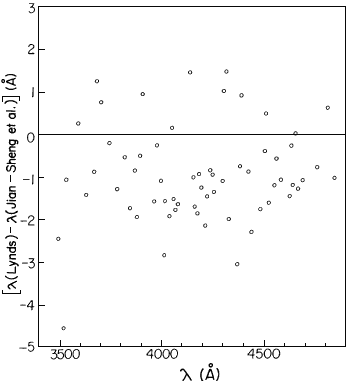
Fig.1. The wavelength difference between the wavelengths of
Lynds and those of
Jian-sheng et al. as a function of wavelength.
In Figure 1, we show the difference [(Lynds) -
(Jian-sheng et al.)] versus for these
64 lines. It will be noted that Lynds's values were systematically too low. The median
of the point shown in Figure 1 is at - 1.07 Ĺ. The r.m.s. departure of Lynds's values
from this line is 1.13 Ĺ. Thus it would appear that Lynds's values had a systematic error
of about 1 Ĺ and a r.m.s. error of 1.13 Ĺ.
To give an idea of the difficulty in identifying lines when the observations have such
large errors, we note that in RMT (Moore, 1945) alone, at about 4000 Ĺ, the number
of possible identifications in an interval of ± 2 Ĺ is about 30 . And we should not forget
that a lot of new data have accumulated since RMT was compiled.
(c)
Coleman (1978)
and
Jian-sheng et al. (1981)
The region 3410 to 5000 Ĺ is common to the observations of
Coleman (1978)
and
Jian-sheng et al. (1981).
In this region, Coleman found 135 lines, while
Jian-sheng et al.,
186. A comparison of the two sets shows that
Jian-sheng et al.'s
results divide Coleman's lines as follows : 6 lines resolved in two, one resolved in three. There was
blending of two lines at two places. Sixteen Coleman lines were not confirmed ; most
of these were weak lines. Sixty-one new lines were found, not all of them are weak : 3
have W > 3, 3 have 3 < = W < = 2, and 28 have
2 < W < = 1 (all in Ĺ). While the claimed
resolution is approximately the same in two cases, it appears that there were some
important shortcomings in the techniques used by
Coleman (1978)
which led to the non-detection of so many lines.
From the above discussion it is obvious that the resolution alone is not an adequate
indicator of the quality of the reported spectrum. It is desirable that the signal-to-noise
ratio also be given in observational papers.
A comparison of the common lines between Coleman and
Jian-sheng et al.
shows that the ratio
W(Jian-sheng et al.)/W(Coleman)
varies between 1 and 7. One, of course,
has to remember that the equivalent widths depend on how the continuum is drawn.
We wish to emphasize the large discrepancies in the equivalent widths given by different
observers to indicate that for the purpose of identification of lines the recorded
equivalent widths can only be taken as a qualitative guide and no more.
The progressive increase in the number of observed lines - 93 (Lynds), 135
(Coleman),
and 203
(Jian-sheng et al.)
- with the improvement in observational
technique clearly indicates that even the list of
Jian-sheng et al.
is not complete and this
factor has to borne in mind while considering the number of lines of any element which
are identified as against the expected number of lines. This also applies to the question
of completeness of multiplets in the identifications. In addition, one has to remember
that in the spectra of stars it is known that `mutilated multiplets' do occur.
The tolerance (or wavelength discrepancy) that one can permit in the identifications
depends on the resolution, uncertainty in the wavelength calibration and the width of
the line. The claimed resolution in the work of
Jiang-sheng et al. (1981)
is 2 Ĺ which would suggest a tolerance of about 1 Ĺ, provided the two adjacent lines are of equal
intensity, which would not be the case in general. The wavelength calibration of
Jian-sheng et al.
was quite good, residuals being 0.1 Ĺ for 3700 Ĺ but up to 0.2 Ĺ at
shorter wavelengths. The widths of the lines arising from the limitations of the
instrumentation and/or blending poses a more serious problem. An examination of an
enlargement of the spectrum shown in Figure 1 of
Jian-sheng et al. (1981)
shows that there are a good many lines having a width greater than 2 Ĺ. Sometimes a blend is
several Angstroms wide. Clearly in such cases a tolerance commensurate with the width
has to be allowed. In the light of the above discussion we have taken 1.5 Ĺ as a guiding
value for the tolerance but larger values have been allowed in appropriate situations.
Identifications for most of the absorption lines in the region shortward of 5000 Ĺ
reported by
Jian-sheng et al. (1981) are presented in
Table II.
Beyond 5000 Ĺ the
available data are very unsatisfactory. Only two sets are available, those of
Lynds (1971) and
Jian-sheng et al. (1981),
and there are serious disagreements between the two sets.
Also for identification purposes the requirements on accuracy become more demanding
in this region - the reason being that most of the lines in this region arise from excited
states and are generally weak as compared to those at shorter wavelengths . Because of
this, we have not even attempted to propose any identifications for lines in this region.
For judging the relative intensities of lines for identification purposes, we have taken
as our guide the relative intensities of those lines in the spectra of shell stars
(
Struve and Roach, 1939.
Struve and Swings, 1941,
1943;
Baldwin, 1941a,
b,
1943.
Struve, 1943;
Broyles, 1943;
Hiltner, 1944;
Merrill and Sanford, 1944;
Weaver, 1952;
Merrill and Lowen, 1953;
Ballereau, 1980),
rather than the laboratory intensities listed in Moore (1945).
The reported equivalent widths of lines in 0805+046 appear to indicate that in
some cases, besides the proposed identifications, there is blending due to unknown
components. The r.m.s. value of (obs-iden.) for all the identifications is 1.24 Ĺ which
is quite satisfactory.
Next we shall consider some of the identified ions.
He I.
A great many lines are present. The only important line missing is 4026.
Mg I
3829, 3838 are present but 3832 is absent. This is, however, not surprising.
The lower level of 3832 is not strictly metastable (Struve, 1939;
Baldwin, 1941) and
this line is sometimes absent in the spectra of shell stars
(Baldwin, 1941).
Mg II
The well-known line 4481 is present.
Si II
Multiplets 1 and 3 are present.
Ca II
Part of the equivalent widths of K and H lines is expected to be interstellar.
Sc II
Scandium is a rare element, but 4247 attains considerable strength in a few
shell stars. 4247 is present here. In addition, most members of multiplets 2 and 3 are
present.
FeII
Many members of multiplets 27, 28, 37, and 38 are present.
The observed line at 4225 deserves special mention. The tracing given by
Jian-sheng et al. (1981)
shows it to be a strong, wide, and slightly asymmetrical line. The width at
half intensity is about 7 Ĺ. Ca I 4226 has been included in the identification of this line
because of its strong intensity. It could, of course, be argued that at the level of excitation
indicated by other ions, Ca I is unlikely to be present. However, there may be stratification
in the shell. The problem can be resolved by higher resolution observations.
Next Section: Conclusion